A Simple Loss Function for Multi-Task learning with Keras implementation, part 2
In this post, we show how to implement a custom loss function for multitask learning in Keras and perform a couple of simple experiments with itself. TL;DR; this is the code:
kb.exp(
        kb.mean(kb.log(kb.mean(kb.square(y_pred - y_true), axis=0)), axis=-1))
In a previous post, I filled in some details of recent work on on multitask learning. Here I will describe a few experiments to investigate the applicability of the new loss function described therein and show an implementation in Keras, a Python library for neural networks. Let’s start with a set of tasks that ideally fulfill the assumptions under which the loss function was derived and show the increase in performance over regular MSE. A different example that doesn’t fit so well the assumptions will follow. Only the ML-related code is shown here, but the rest is available
Learning the \(\sin\) function with noise
Let’s keep it simple by choosing to learn the \(\sin\) function in the \([0,
2\pi]\) interval with different amounts of gaussian noise added. The first
task is generating some data to feed into this experiment. Let’s sample the
independent variable to randomly in the \([0,1]\) interval, then pick 5
numbers to use as standard deviations and then draw from normal distributions
with 0 means and these standard deviations to obtain 5 progressively more
noisy versions of the original task. Finally, let’s add two columns with the
values of the independent variable and the original, noiseless dependent
variable values, for ease of plotting (np is short for numpy and pd for
pandas):
def make_data_hetero():
    """Generate data for the heteroscedastic multitask learning experiment.

    Returns
    -------
    DataFrame
        One column per learning task, increasing noise

    """
    xx = np.random.uniform(0, 1, N)
    y = [math.sin(x * 2 * math.pi) for x in xx]

    sds = [.1 * 2**i for i in range(0, n_tasks)]
    data = pd.DataFrame(
        {i: y + np.random.normal(0, sds[i], N)
         for i in range(len(sds))})
    data.columns = ["y" + str(c) for c in data.columns]
    data["x"] = xx
    data["y"] = y
    return data


data_hetero = mtl.make_data_hetero()
Let’s take a look: there are 7 columns, 5 with the dependent variables, which will be the learning target, simulatneously for a single model; one for the dependent variable; and one for the noiseless values on which the five tasks are based:
| y0 | y1 | y2 | y3 | y4 | x | y |
|---|---|---|---|---|---|---|
| 0.60 | 0.28 | 0.12 | -0.63 | 0.46 | 0.42 | 0.50 |
| -0.96 | -0.86 | -1.04 | -2.11 | 0.33 | 0.72 | -0.98 |
| -0.14 | 0.01 | 0.26 | -0.35 | -0.61 | 0.00 | 0.00 |
| 1.01 | 0.73 | 1.04 | 2.41 | -1.59 | 0.30 | 0.95 |
| 0.83 | 0.83 | 0.76 | 0.48 | 1.58 | 0.15 | 0.80 |
While discussing multitask learning is not the goal here, this is a favorable setting for it, with 5 closely related tasks in that the noiseless function to be learned is the same for all the tasks. But the 5 tasks are also different since they are progressively more noisy, a problem the multitask loss here presented is designed to tackle. Let’s split the data in train, test and stop data set. I need a stop dataset because I plan to use early stopping to protect against overfitting, but in many papers the test set is used for such purpose. I believe a true test set and a learning algorithm need to have an “air gap” for the test set to fulfil its task, as many Kaggle competitions have amply demonstrated.
def split_data(data):
    """Split a dataset in three chunks in 1:9:10 proportions.

    Parameters
    ----------
    data : type
        DataFrame to split.

    Returns
    -------
    type
        A tuple with three data frames.

    """
    N = data.shape[0]
    return data[0:N // 20], data[N // 20:N // 2], data[N // 2:N]

data_hetero_train, data_hetero_stop, data_hetero_test = mtl.split_data(
    data_hetero)
The reader may have noticed that stop and test sets are much bigger then the training set. I wanted to keep the task difficult but have reliable ways to avoid overfitting and to evaluate the effect of the change in loss function, which is the only goal of this exercise. In practice, such a split is not commonly used.
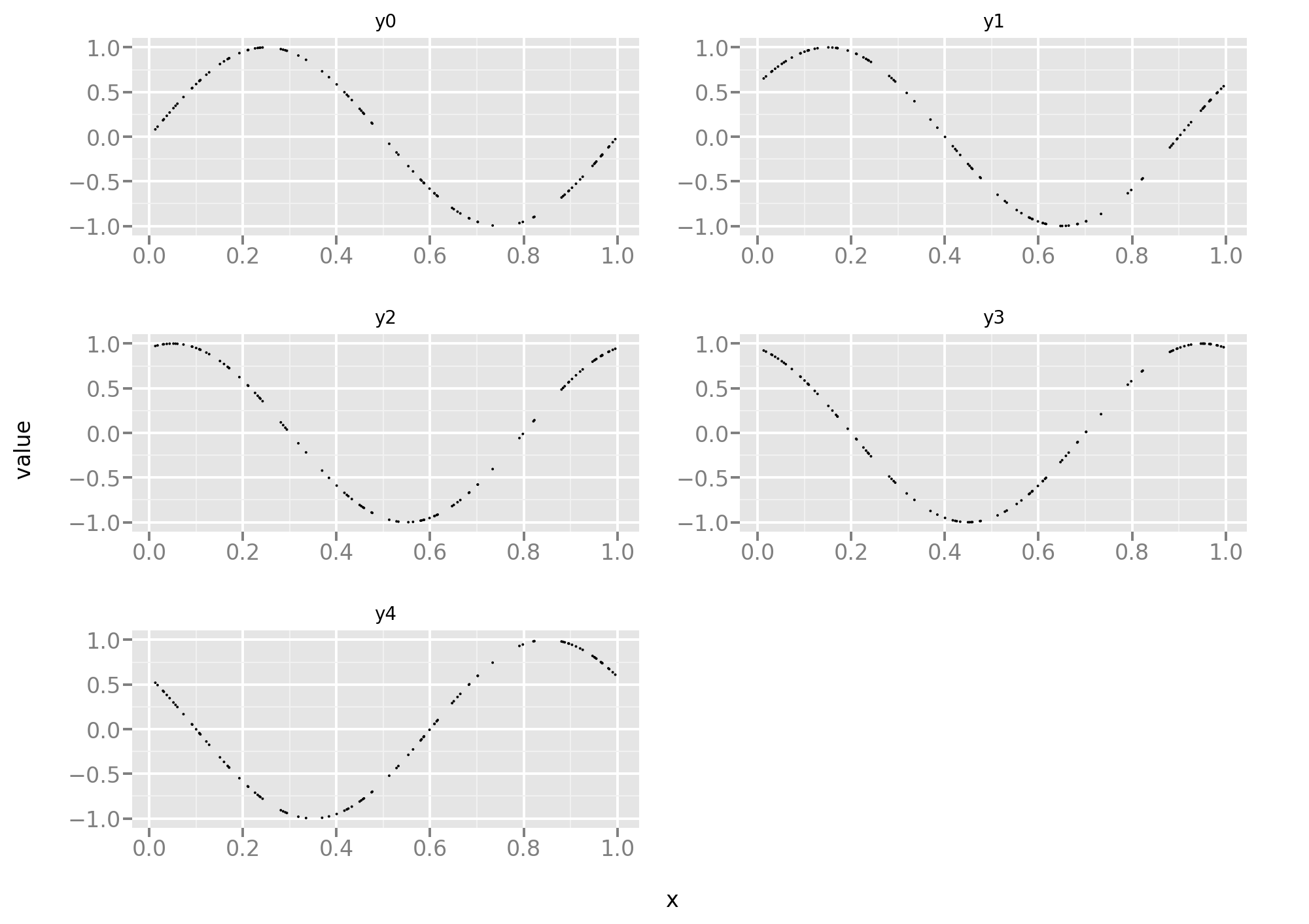
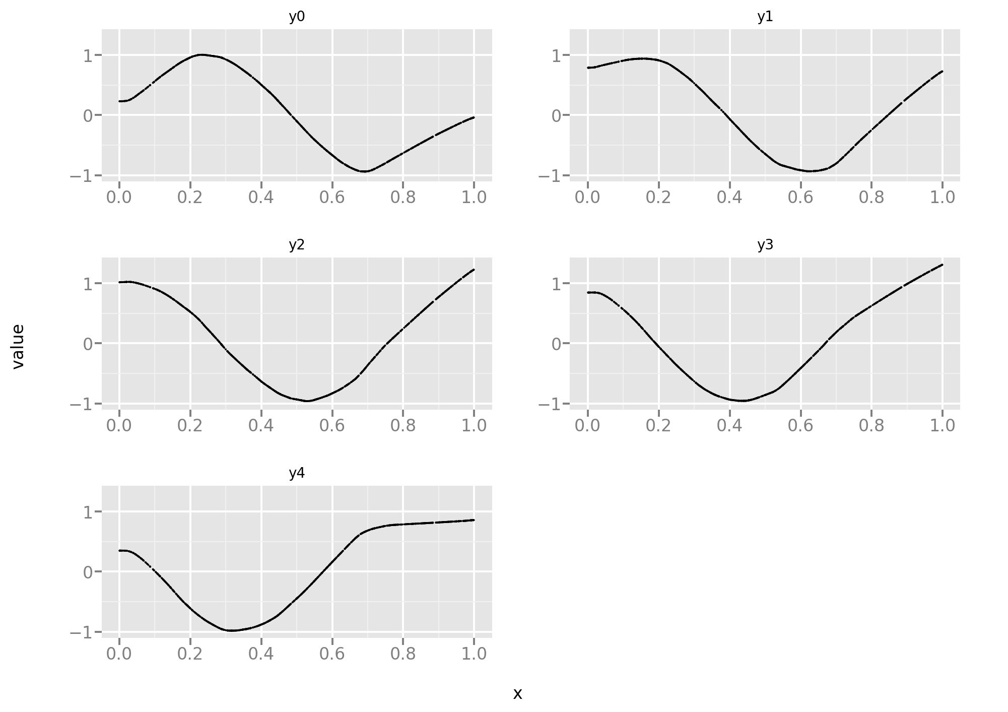
First let’s take a peek at the training set:
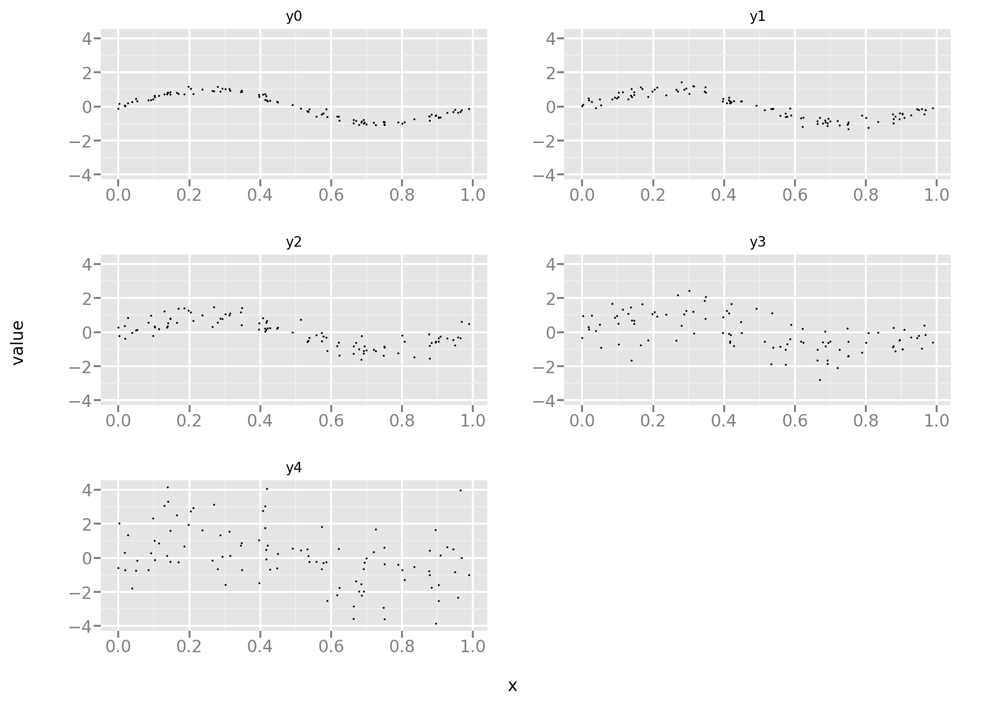
As one can see, progressively more noisy versions of the same task.
Let’s now define a neural net model. I picked a multi-layer perceptron with
10 layers so as to allow enough steps for the tasks to be solved in an
integrated fashion. One big novelty about deep
learning
is the possibility to share internal
representations
between tasks, whereas with shallow models, neural or not, this is not
possible. I did not tinker much with sizing, since I didn’t want to bias the
results of the experiments. One thing I did tinker with a little,
reluctantly, were the patience parameter in the early stopping rule and
the epsilon parameter in the Adam optimizer. This was to counter a
pernicious tendency of the optimization to reverse course, that is increase
the loss, sometimes drastically so, towards the end of the fitting process.
Apparently the Adam optimizer is
prone, when gradients are
very small, to running into numerical stability issues, and increasing the
epsilon parameter helps with that, while slowing the learning process.
Increasing the patience parameter has the effect of continuing the
optimization even when plateaus of very low gradient are reached.
Decreasing it results in the fitting process to stop before it has reached a
local minumum, because of the randomness intrinsic to Stochastic Gradient
Descent, on which Adam is based. It is unfortunate that many if not all of
these optimizers have so many knobs that may need to be accessed to achieve
good performance. Not only are they laborious to operate, but they can also
get us lost in Andrew Gelman’s so-called Garden of Forking
Paths,
whereby overfitting can occur more or less unintentionally. The importance of
this is starting to be
recognized by
the most alert members of the ML community, but is a well established theme
in statistics (multiple testing correction, false discovery rate etc.)
def NN_experiment(data_train, data_stop, loss):
    """Fit a model.

    Parameters
    ----------
    data_train : DataFrame
        Data to train on.
    data_stop : DataFrame
        Data to use for early stopping.
    loss : Function
        Loss function to use.

    Returns
    -------
    Tuple of Keras Model and hist object
        Tuple with fitted model and history of fitting process.

    """
    U = 100
    L = 10
    NN = K.models.Sequential([
        K.layers.Dense(
            input_shape=(1, ), units=U, activation=K.activations.relu)
    ] + [
        K.layers.Dense(units=U, activation=K.activations.relu)
        for _ in range(L - 1)
    ] + [K.layers.Dense(n_tasks, activation="linear")])
    NN.compile(optimizer=K.optimizers.Adam(epsilon=1E-3), loss=loss)
    hist = NN.fit(
        x=data_train["x"].values,
        y=data_train.iloc[:, range(0, n_tasks)].values,
        epochs=200,
        callbacks=[K.callbacks.EarlyStopping(patience=5)],
        validation_data=(data_stop["x"].values,
                         data_stop.iloc[:, range(0, n_tasks)].values),
        verbose=0)
    return (NN, hist)

NN_hetero_mse, hist_hetero_mse = mtl.NN_experiment(
    data_hetero_train, data_hetero_stop, kl.mean_squared_error)
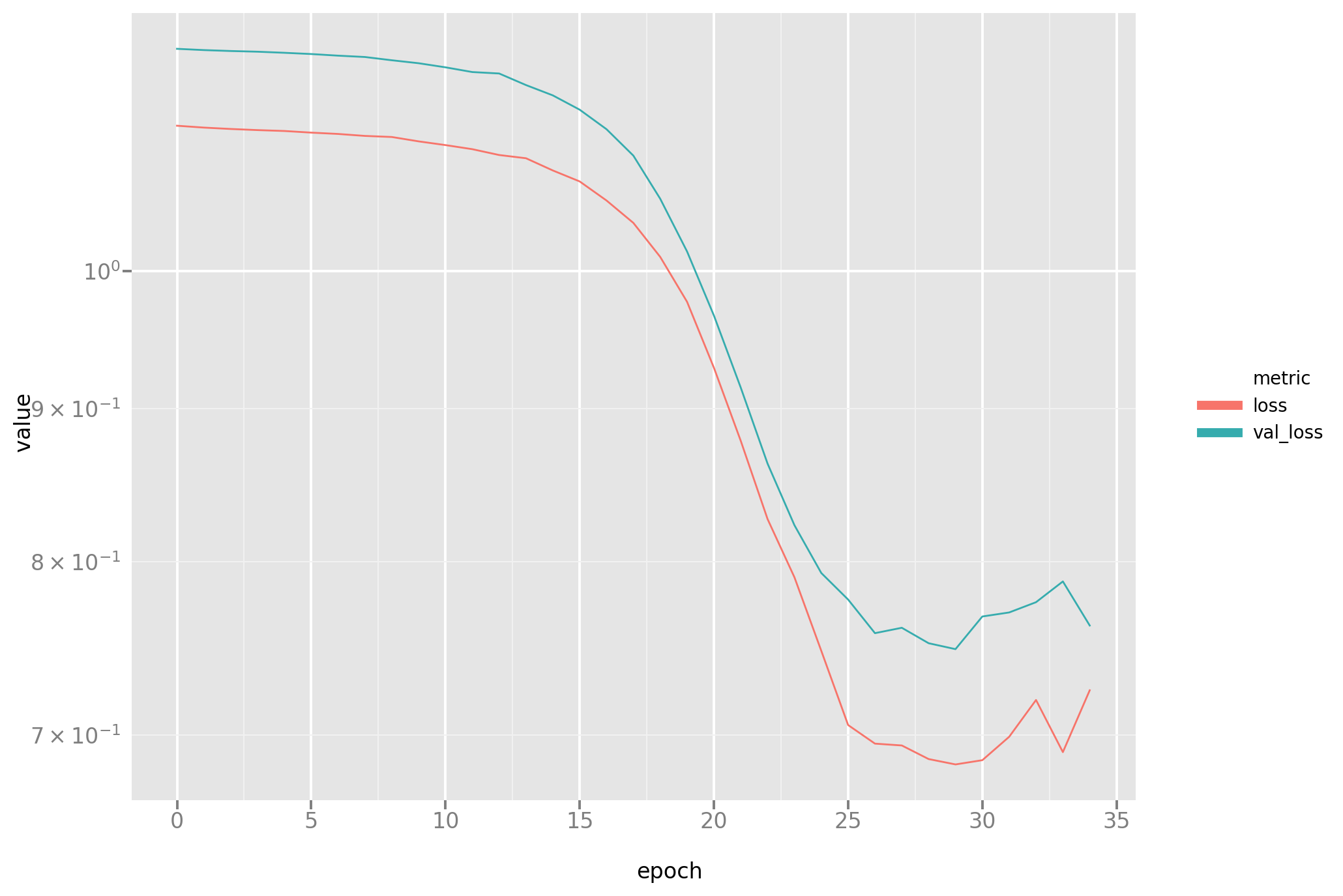
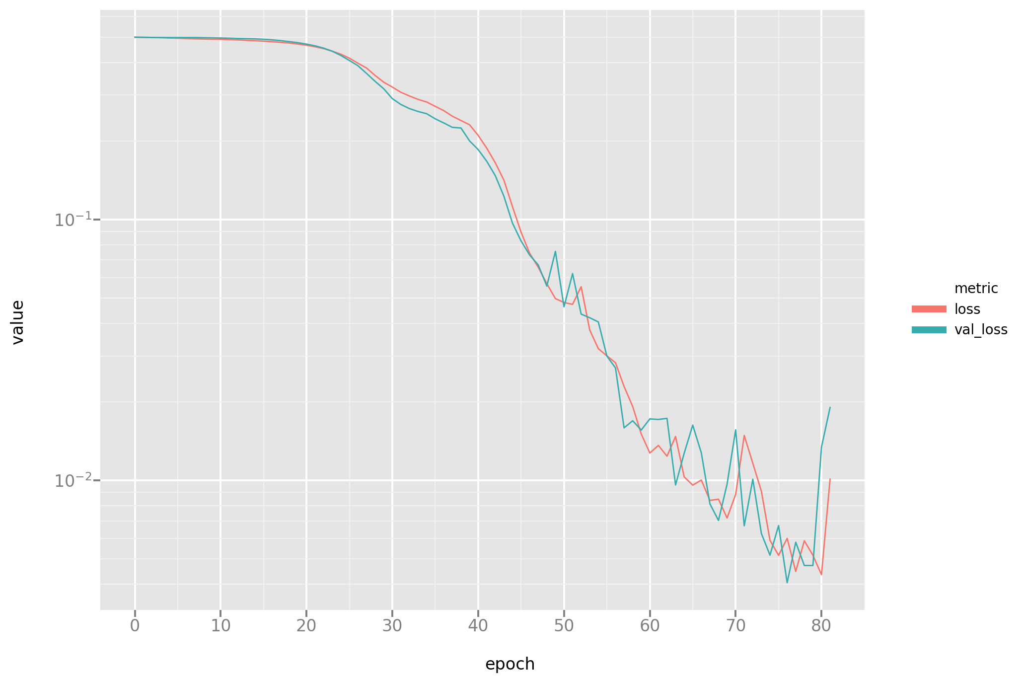
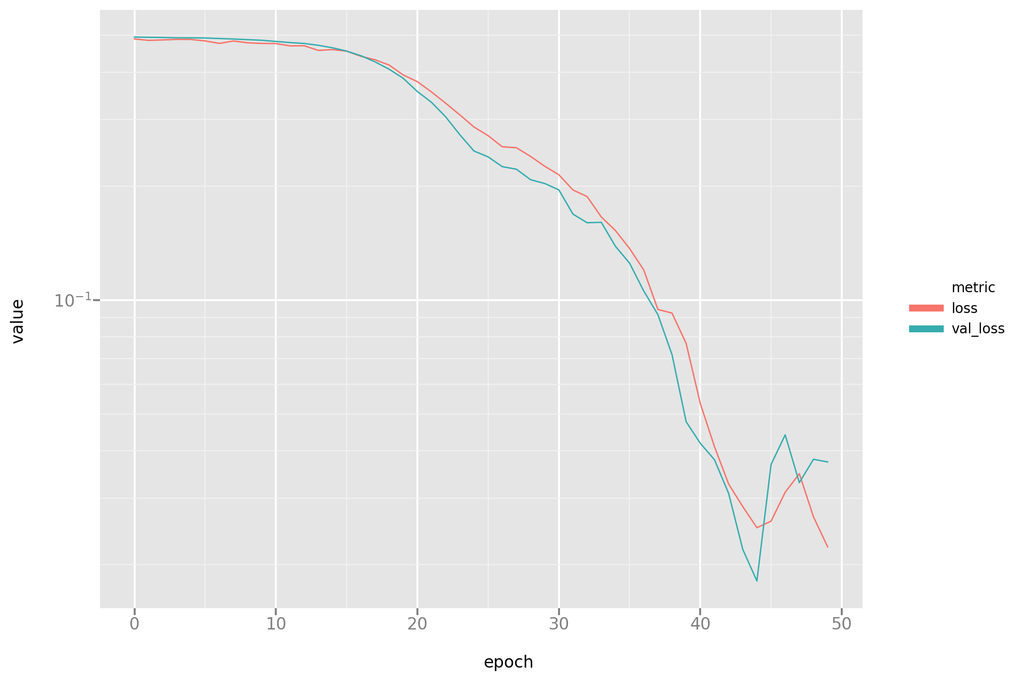
In addition to the fitted model, a record of the training process is also
being stored, which enables a standard visualization of how training set and
stop set losses (named loss and val_loss resp. in the graph) decrease
over the epochs of training. Also please note how this function is
parametrized on the loss function, which will enable the central comparison
in this post.
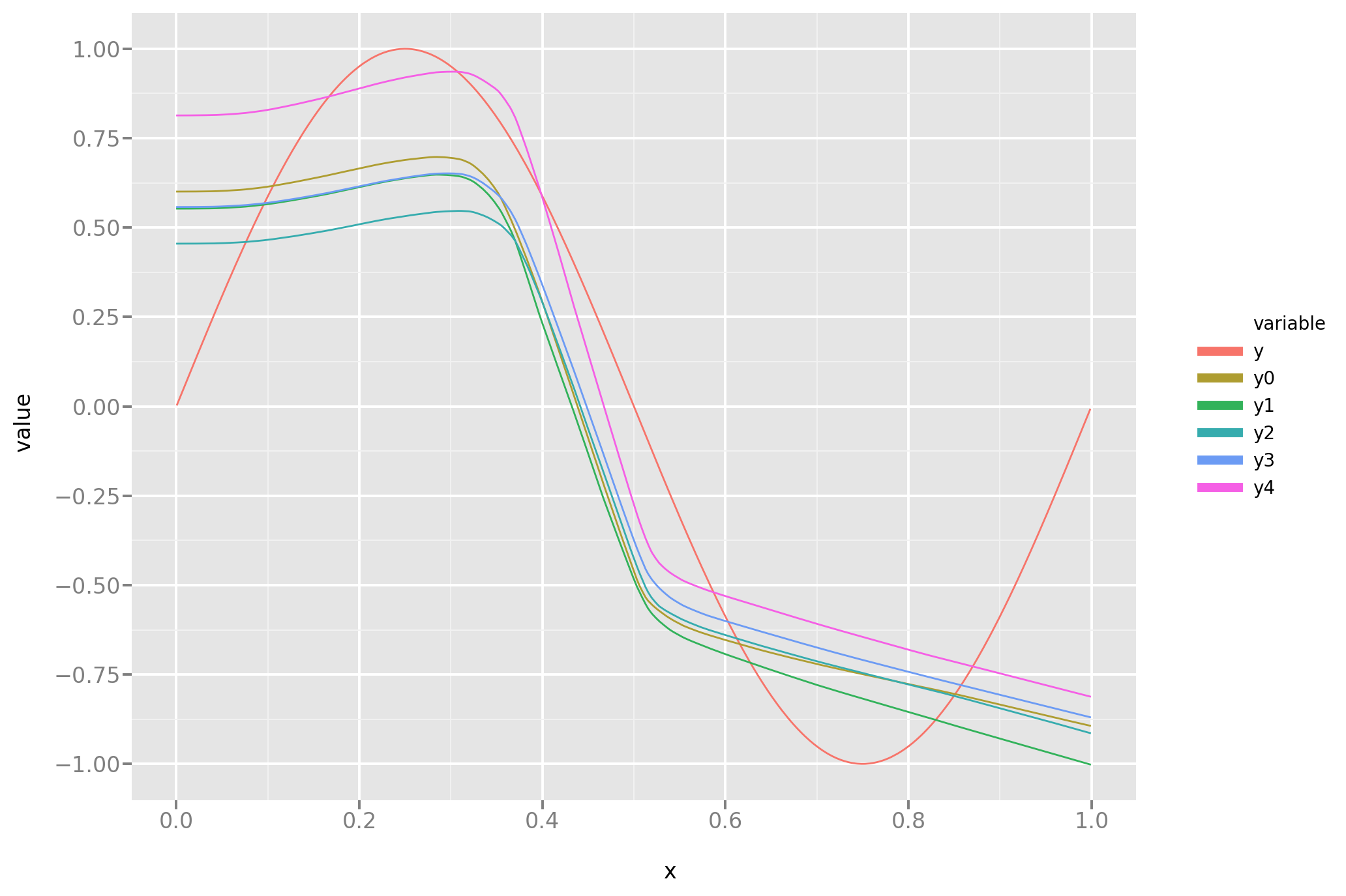
And here is a look at the actual predictions. A more rigorous comparison between this and the novel approach will follow.
Now let’s repeat this is experiment substituting the standard MSE loss with the one derived in the previous post on this subject. As the reader can see, the implementation in Keras is simple but one has to substitute standard vector operations with Keras low level ones, and make sure to use the correct axis when operating on tensors.
def mean_squared_error_hetero(y_true, y_pred):
    """Loss function for multitask learning.

    Parameters
    ----------
    y_true : tensor
        The target value/
    y_pred : tensor
        The predicted value.

    Returns
    -------
    tensor
        Distance.

    """
    return kb.exp(
        kb.mean(kb.log(kb.mean(kb.square(y_pred - y_true), axis=0)), axis=-1))

NN_hetero_mseh, hist_hetero_mseh = mtl.NN_experiment(
    data_hetero_train, data_hetero_stop, mtl.mean_squared_error_hetero)
The same loss plot as before for completeness:
And the line plot:
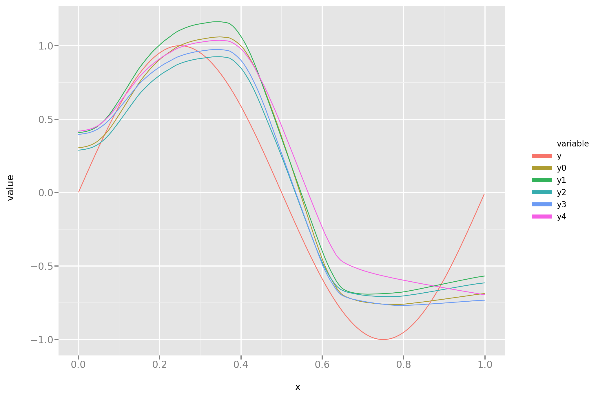
Is it better? Let’s look into it:
def compare_performance(NN1, NN2, data_test, target):
    """Compare performance of two models.

    Parameters
    ----------
    NN1 : keras model
        First  model to compare.
    NN2 : keras model
        Second model to compare.
    data_test : type
        Data to perform comparison  on.
    y : Pandas series
        Ground truth.

    Returns
    -------
    Series
        MSE for each prediction task.

    """
    return pd.DataFrame([
        make_pred(NN, data_test["x"]).subtract(target, axis=0).pow(2).mean()
        for NN in (NN1, NN2)
    ]).drop(
        "x", axis=1)

cperf = mtl.compare_performance(NN_hetero_mse, NN_hetero_mseh,
                                data_hetero_test, data_hetero_test["y"])
And, comparing task by task, it looks like it mostly is:
cperf.iloc[0] / cperf.iloc[1]
y0    1.64
y1    1.77
y2    2.67
y3    1.80
y4    0.86
dtype: float64
The most alert readers for sure are aware of the reproducibility crisis in the sciences, whereby many published results do not stand the test of time. This is a complex subject, but one important factor is that sometimes surprising and interesting and therefore very publishable results occur by chance. Sometimes luck is enhanced, deliberately or not, by the researcher, operating on various analysis “knobs” or discarding “bad data” (also known with the suave term of “data cleaning”) or modifying the metric of interest or the research question until something “interesting” but random shows up. The reviewing and publication process creates the wrong incentives by insisting more on novelty than methodological rigor. In AI research this problem is compounded by frantic competition, automation of hyperparameter search and by the dominance of a few very prominent benchmark datasets that have been studied in depth, thereby leaving no data to be used as a true test set anymore. In this post, working on a small synthetic dataset, there is the opportunity to repeat the experiment many times and estimate the results’ variability:
def one_replication(make_data):
    """Perform one replication of the loss function comparison.

    Parameters
    ----------
    make_data : function
        Generator for data to perform the experiment on.

    Returns
    -------
    Series
        MSE ratio, task by task.

    """
    data = make_data()
    data_train, data_stop, data_test = split_data(data)
    NN_mse, _ = NN_experiment(data_train, data_stop, kl.mean_squared_error)
    NN_mseh, _ = NN_experiment(data_train, data_stop,
                               mean_squared_error_hetero)
    cperf = compare_performance(NN_mse, NN_mseh, data_test, data_test["y"])
    return cperf.iloc[0] / cperf.iloc[1]

pass  # ignore this line
def many_replications(make_data, n=100):
    """Perform many replications of the loss comparison.

    Parameters
    ----------
    make_data : Function.
        Data generator for experiment.
    n : int
        Number of replications.

    Returns
    -------
    DataFrame
        MSE ratio, one col per task, one row per replication.

    """
    return pd.DataFrame([one_replication(make_data_hetero) for _ in range(n)])

pstats_hetero = mtl.many_replications_(mtl.make_data_hetero)
pstats_hetero.plot.box(logy=True)
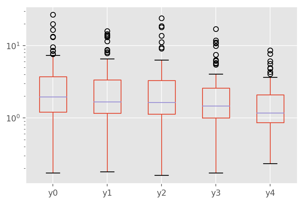
This provides a better understanding of how the new loss function helps in a majority of cases, but can also hurt sometimes. In a practical application, this level of variability would likely not be welcome and would need to be mitigated by training on more data, averaging models over serveral runs or other means.
Learning the \(\sin\) function with multiple phases
Let’s now apply the same techniques to a problem where, like in many AI problems, the challenge is not randomness in the data but just the complexity of the tasks. Specifically, let’s fit a neural model to 5 shifted versions of the the \(\sin\) function, with no added noise.
def make_data_phase():
    """Generate data for the multiphase example.

    Returns
    -------
    DataFrame
        Data f.

    """
    xx = np.random.uniform(0, 1, N)
    data = pd.DataFrame({
        "y" + str(i):
        [math.sin((x * 2 + float(i) / n_tasks) * math.pi) for x in xx]
        for i in range(n_tasks)
    })
    data["x"] = xx
    return data

data_phase = mtl.make_data_phase()
The data split is exactly as before:
data_phase_train, data_phase_stop, data_phase_test = mtl.split_data(data_phase)
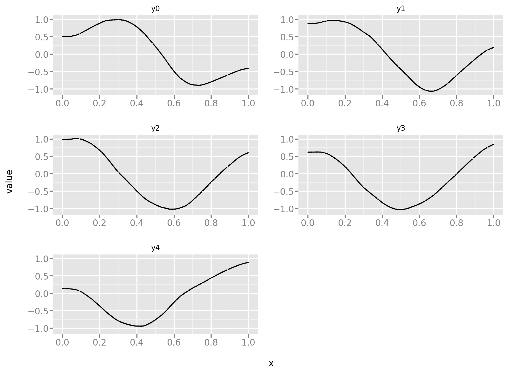
Let’s take a look at the training data. Here the 5 tasks are equally difficult and, since the data is noise-free, it’s more a function approximation problem than a statistical problem.
Let’s reuse the same code as in the first part of this post, starting with the standard MSE loss:
NN_phase_mse, hist_phase_mse = mtl.NN_experiment(
    data_phase_train, data_phase_stop, kl.mean_squared_error)
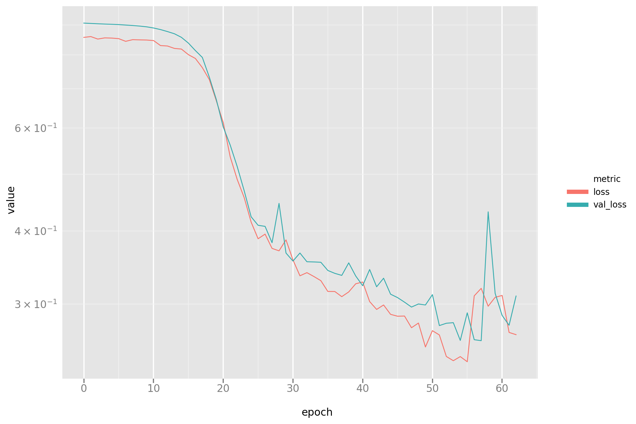
Let’s take a look at the loss dynamic to diagnose any problems in the fitting process:
Next, let’s take a look at the results:
The next run differs only in the choice of loss function:
NN_phase_mseh, hist_phase_mseh = mtl.NN_experiment(
    data_phase_train, data_phase_stop, mtl.mean_squared_error_hetero)
A look at the loss plot (please note some instability at the end of the process, as noted before a known problem with the Adam optimizer)
And a look at the predictions:
They don’t look great and a quantitative assessment confirms that impression:
cperf = mtl.compare_performance(NN_phase_mse, NN_phase_mseh, data_phase_test,
                                data_phase_test)
cperf.iloc[0] / cperf.iloc[1]
y0    0.76
y1    1.56
y2    0.72
y3    0.13
y4    0.17
dtype: float64
Was it a fluke or a reliable comparison? Let’s use replication to answer this question:
pstats_phase = mtl.many_replications_(mtl.make_data_phase)
pstats_phase.plot.box(logy=True)
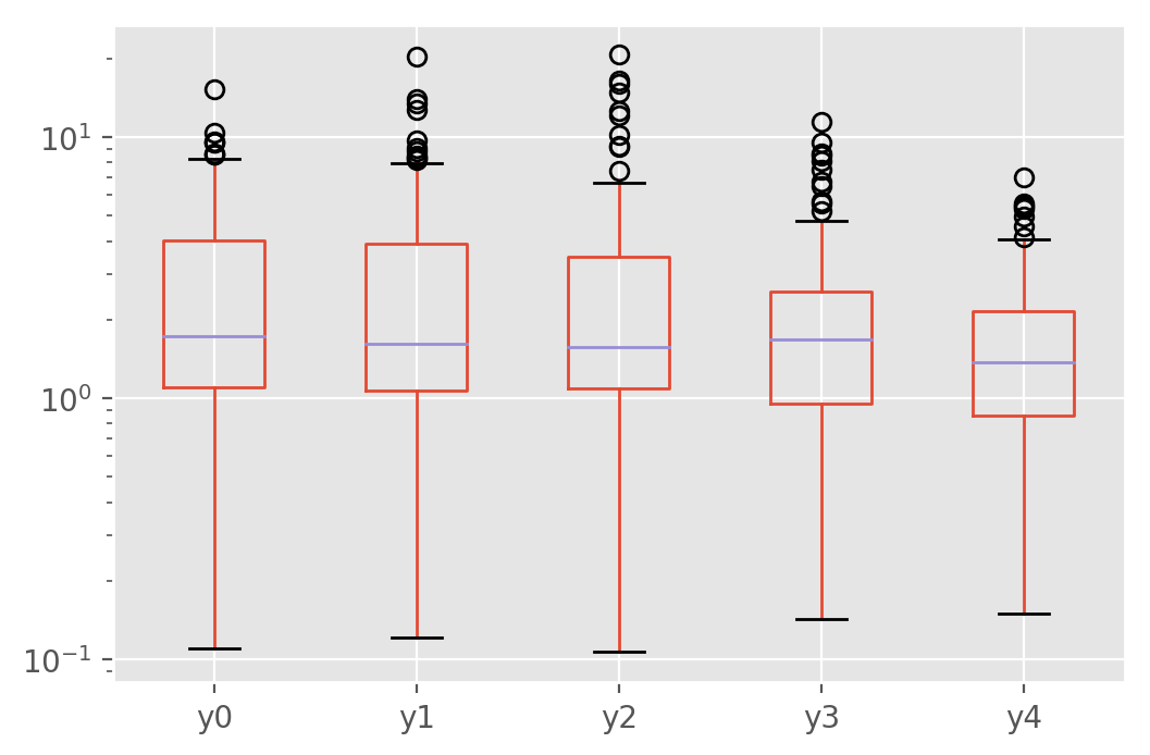
It does indeed look like the first run was not particularly representative. The boxplot shows instead that the multitask loss outperforms the MSE loss even when there is no statistical difference between the tasks in this particular example.
Conclusions
The multitask loss outperforms, on average, the MSE in both of the multitask learning examples presented here. Variability over several, independent datasets is a concern, and is addressed here by reporting statistics over many replications, hopefully representing a budding trend in ML research and practice. While these conclusions do not generalize to other tasks or neural architectures, they provide additional evidence outside the first paper in which the multitask loss was proposed. The underlying theory does not explain why this loss should be the best performer in the second example in this post, for which fitting additional variance parameters seems an unnecessary burden with no clear advantage. But, as it often is the case with neural networks and stochastic gradient descent, experiments seem to be a step or two ahead of theory. The closed form solution for variance parameters in the multitask loss paves the way for a very simple implementation with no performance penalty, and Keras provides intuitive primitives to perform the calculations on a variety of platforms.